Normal Distribution Bell Curve Generator
Free online Normal Distribution Bell Curve generator: get a fully labeled figure in about 90 seconds. The AI plans the must-have label list first, then renders a clean textbook-style diagram — every label editable afterwards, ready for papers, assignments and slides.
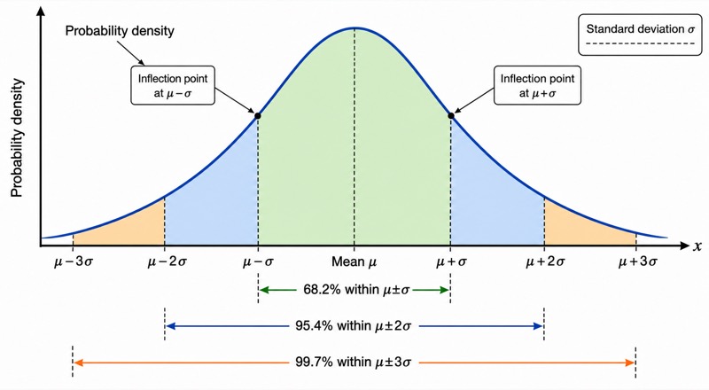
Labels included in this diagram
- Probability density
- μ-3σ
- μ-2σ
- μ-σ
- Mean μ
- μ+σ
- μ+2σ
- μ+3σ
- Standard deviation σ
- 68.2% within μ±σ
- 95.4% within μ±2σ
- 99.7% within μ±3σ
- Inflection point at μ-σ
- Inflection point at μ+σ
✓ Accurate labels ✓ Edit text after generation ✓ PNG for papers, posters & slides
 OUTPUT · 16:9 · PNG
What this diagram shows
A normal distribution diagram shows a continuous, symmetric probability distribution centered at the mean μ. The horizontal axis represents values measured in standard-deviation units from the mean, typically from μ − 3σ to μ + 3σ, while the vertical axis represents probability density rather than probability itself. The bell-shaped curve reaches its maximum at μ, where the mean, median, and mode coincide. Its two tails decrease smoothly and approach, but never touch, the horizontal axis. Shaded regions under the curve illustrate the empirical rule: approximately 68.2% of observations lie within one standard deviation, 95.4% within two, and 99.7% within three.
Standard deviation σ controls the horizontal spread of the curve: a larger σ produces a wider, flatter bell, whereas a smaller σ produces a narrower, taller bell when total area remains 1. The points μ − σ and μ + σ are the inflection points, where the curve changes from concave downward to concave upward. The central 68.2% region extends from μ − σ to μ + σ. Adding the next two bands gives 95.4% between μ − 2σ and μ + 2σ, and adding the outer bands gives 99.7% between μ − 3σ and μ + 3σ. Symmetry means corresponding left and right bands have equal areas.
What a correct diagram must include
- A symmetric bell-shaped curve: draw identical left and right halves around μ so equal deviations from the mean have equal density.
- A clearly labeled horizontal axis: mark μ − 3σ, μ − 2σ, μ − σ, μ, μ + σ, μ + 2σ, and μ + 3σ at equal intervals.
- The mean μ at the center and peak: place μ directly below the highest point because the mean, median, and mode coincide in a normal distribution.
- Inflection points at μ − σ and μ + σ: identify these as the locations where the curvature changes, not where the curve reaches zero.
- Nested empirical-rule intervals: show 68.2% within ±1σ, 95.4% within ±2σ, and 99.7% within ±3σ without treating the percentages as separate totals.
- Area-based shading: shade regions under the curve, because probability is represented by area rather than by the height of the curve.
- Equal subdivisions on both sides: if individual bands are labeled, use about 34.1%, 13.6%, and 2.15% from the center outward on each side.
- Tails extending beyond ±3σ: continue the curve past the displayed interval and make it approach the axis asymptotically, since about 0.3% of the area lies outside ±3σ.
Common mistakes
- Labeling the axis simply −3σ to +3σ when it represents raw values; use μ − 3σ through μ + 3σ, or use z-scores −3 through +3 for the standard normal distribution.
- Placing the inflection points at μ ± 2σ or at the ends of the curve; for a normal density, they occur exactly at μ ± σ.
- Adding 68.2%, 95.4%, and 99.7% as separate regions; these are nested cumulative intervals centered at μ.
- Making the curve touch the horizontal axis at ±3σ; normal-distribution tails extend indefinitely and only approach the axis.
- Interpreting curve height as the probability of an exact value; for a continuous distribution, probabilities come from areas over intervals, and any single exact value has probability zero.
Teaching tips
Use the diagram after introducing mean, variance, and standard deviation, or before exercises on z-scores and normal probabilities. Ask students to locate μ ± kσ, identify the inflection points, and estimate the proportion inside or outside a stated interval. Follow with questions such as, “What percentage lies between μ + σ and μ + 2σ?” or “What proportion is above μ + 2σ?” The figure supports assessment of symmetry, complementary probability, the empirical rule, standardization, and the distinction between density height and area under a continuous probability curve.
FAQ about this diagram
Why are μ − σ and μ + σ called inflection points?
At these points, the normal density changes curvature from concave downward near the center to concave upward in the tails. They also mark one standard deviation from the mean, but they are not boundaries of the distribution.
Do 68.2%, 95.4%, and 99.7% apply to every bell-shaped data set?
No. These percentages are the empirical rule for a normal distribution and are only approximations for data that are approximately normal. Skewed, multimodal, or heavy-tailed distributions may differ substantially.
How can the percentage between two adjacent standard-deviation marks be found?
Subtract nested central areas and divide by two because of symmetry. For example, the area from μ + σ to μ + 2σ is approximately (95.4% − 68.2%)/2 = 13.6%, while the area from μ + 2σ to μ + 3σ is about (99.7% − 95.4%)/2 = 2.15%.