Neural Network Architecture Diagram (CNN) Generator
Free online Neural Network Architecture Diagram (CNN) generator: get a fully labeled figure in about 90 seconds. The AI plans the must-have label list first, then renders a clean textbook-style diagram — every label editable afterwards, ready for papers, assignments and slides.
Labels included in this diagram
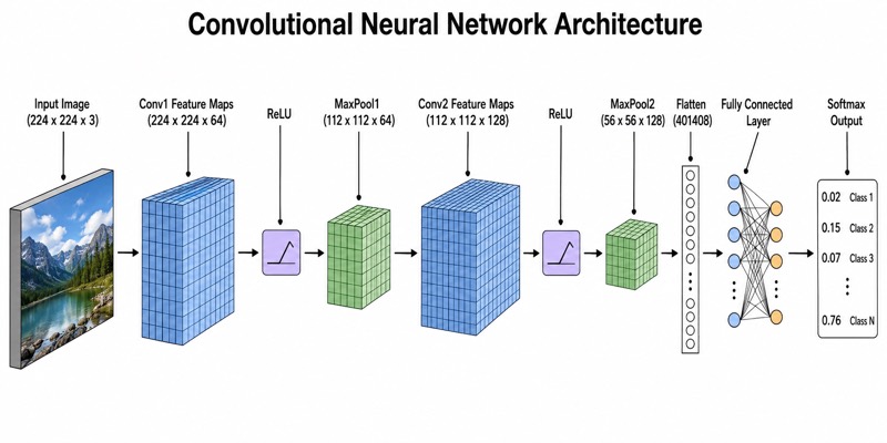
- Input Image (224 x 224 x 3)
- Conv1 Feature Maps (224 x 224 x 64)
- ReLU
- MaxPool1 (112 x 112 x 64)
- Conv2 Feature Maps (112 x 112 x 128)
- ReLU
- MaxPool2 (56 x 56 x 128)
- Flatten (401408)
- Fully Connected Layer
- Softmax Output
✓ Accurate labels ✓ Edit text after generation ✓ PNG for papers, posters & slides
 OUTPUT · 16:9 · PNG
What this diagram shows
This CNN architecture diagram represents the forward propagation of an image classification network. The Input Image has dimensions 224 × 224 × 3, where the first two values are spatial dimensions and 3 denotes color channels. Conv1 produces 64 feature maps of size 224 × 224, typically through same padding, while ReLU introduces nonlinearity. MaxPool1 reduces the spatial resolution to 112 × 112 without changing the channel count. Conv2 then expands the representation to 128 channels, and MaxPool2 reduces each feature map to 56 × 56. The three-dimensional blocks visualize height, width, and channel depth.
Arrows should connect the stages from left to right to show the computational order: Input Image, Conv1 Feature Maps, ReLU, MaxPool1, Conv2 Feature Maps, ReLU, MaxPool2, Flatten, Fully Connected Layer, and Softmax Output. Convolution learns local patterns such as edges, textures, and increasingly complex features. ReLU applies max(0, x) elementwise, and max pooling downsamples each channel by selecting local maximum values. The final tensor contains 56 × 56 × 128 = 401408 activations, which Flatten converts into a one-dimensional vector. The fully connected layer combines these features, and Softmax converts the final logits into normalized class probabilities.
What a correct diagram must include
- Input tensor: Draw a three-dimensional block labeled Input Image (224 × 224 × 3) so height, width, and color-channel depth are explicit.
- Convolution stages: Label Conv1 Feature Maps (224 × 224 × 64) and Conv2 Feature Maps (112 × 112 × 128), showing that convolution changes channel depth while same padding preserves spatial size.
- Activation functions: Place ReLU immediately after each convolution because nonlinear activation enables the network to model relationships beyond linear filtering.
- Pooling stages: Show MaxPool1 (112 × 112 × 64) and MaxPool2 (56 × 56 × 128), making clear that pooling halves height and width but preserves channel count.
- Tensor geometry: Use three-dimensional rectangular prisms whose height, width, and depth visually correspond to the changing feature-map dimensions.
- Forward-propagation arrows: Connect every operation from left to right with directional arrows and avoid arrows that skip required computational stages.
- Flatten transition: Label Flatten (401408) and verify the calculation 56 × 56 × 128 = 401408 before connecting the tensor to the dense stage.
- Classification head: End with a Fully Connected Layer followed by Softmax Output, distinguishing unnormalized logits from normalized class probabilities.
Common mistakes
- Treating 224 × 224 × 64 as 64 separate images rather than one activation tensor containing 64 feature maps.
- Reducing the channel count during max pooling; standard spatial max pooling changes height and width but normally keeps the number of channels unchanged.
- Writing the Flatten size incorrectly; the correct value after MaxPool2 is 56 × 56 × 128 = 401408.
- Placing ReLU before convolution or Softmax before the fully connected output; this reverses the intended forward-propagation sequence.
- Claiming that Softmax learns features; Softmax only transforms output logits into a probability distribution whose values sum to 1.
Teaching tips
Use the diagram after introducing convolution kernels and before discussing model training. Ask students to predict the output shape after each operation, explain why convolution increases channel depth, and calculate the Flatten dimension independently. A useful comparison question is why ReLU changes values but not tensor shape, whereas MaxPool changes spatial dimensions but not channel count. The diagram also supports exam questions on forward propagation, same padding, pooling, tensor-shape calculations, feature hierarchies, logits, and the interpretation of Softmax probabilities.
FAQ about this diagram
Why do the convolution layers preserve spatial dimensions in this diagram?
They are assumed to use same padding with an appropriate stride, usually stride 1. Padding adds border values so the output height and width remain equal to those of the input tensor.
Why does MaxPool reduce width and height but not the number of channels?
Max pooling operates independently within each feature map. A 2 × 2 pooling window with stride 2 halves the spatial dimensions while producing one pooled map for every input channel.
What is the difference between Flatten, the fully connected layer, and Softmax?
Flatten reshapes the 56 × 56 × 128 tensor into a 401408-element vector without learning parameters. The fully connected layer applies learned weights to produce logits, and Softmax normalizes those logits into class probabilities.